Extreme Learning Machine

1,801 Views

Sinopsis

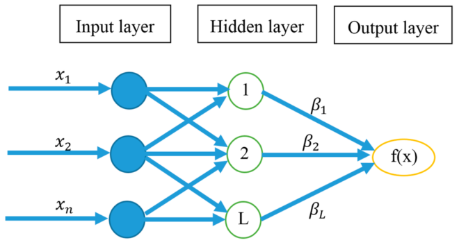
Bila ditemui kasus mengenai non linear selain bisa menggunakan SVM (Support Vector Machine), kita juga bisa menggunakan ELM yaitu The Extreme Learning Machine (ELM from now on) was proposed by [Huang et al., 2006]. It is used in a multilayered structure with one neural hidden layer (Single Layer Feedforward Network, SLFN from now on). The first step is to initialize at random the weights connecting the input and the hidden layer. Thus, it will only be necessary to optimize the weights connecting the hidden layer and the output layer. In order to do this, the Moore-Penrose pseudoinverse [Rao and Mitra, 1972] matrix will be used.

References

[Huang et al., 2006] Huang, G. B., Zhu, Q. Y., and Siew, C. K. (2006). Extreme learning machine: Theory and applications, Neurocomputing, volume 70, 489-501.
[Haykin, 1998] Haykin, S. (1998). Neural Networks: A Comprehensive Foundation. Prentice-Hall.
[Rao and Mitra, 1972] Rao, C. R. and Mitra, S. K. (1972). Generalized Inverse of Matrices and It’s Applications. Wiley.

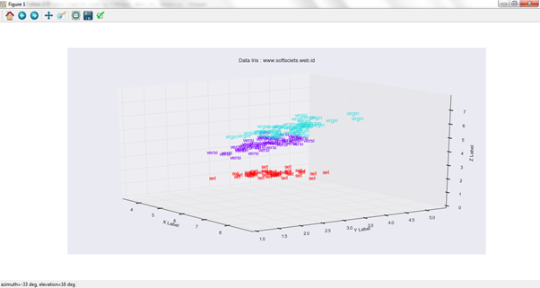
Penulis menggunakan dataset iris sebagai berikut

x1	x2	x3	x4	target
5.1	3.5	1.4	0.2	0
4.9	3	1.4	0.2	0
4.7	3.2	1.3	0.2	0
4.6	3.1	1.5	0.2	0
5	3.6	1.4	0.2	0
5.4	3.9	1.7	0.4	0
4.6	3.4	1.4	0.3	0
5	3.4	1.5	0.2	0
4.4	2.9	1.4	0.2	0
4.9	3.1	1.5	0.1	0
5.4	3.7	1.5	0.2	0
4.8	3.4	1.6	0.2	0
4.8	3	1.4	0.1	0
4.3	3	1.1	0.1	0
5.8	4	1.2	0.2	0
5.7	4.4	1.5	0.4	0
5.4	3.9	1.3	0.4	0
5.1	3.5	1.4	0.3	0
5.7	3.8	1.7	0.3	0
5.1	3.8	1.5	0.3	0
5.4	3.4	1.7	0.2	0
5.1	3.7	1.5	0.4	0
4.6	3.6	1	0.2	0
5.1	3.3	1.7	0.5	0
4.8	3.4	1.9	0.2	0
5	3	1.6	0.2	0
5	3.4	1.6	0.4	0
5.2	3.5	1.5	0.2	0
5.2	3.4	1.4	0.2	0
4.7	3.2	1.6	0.2	0
4.8	3.1	1.6	0.2	0
5.4	3.4	1.5	0.4	0
5.2	4.1	1.5	0.1	0
5.5	4.2	1.4	0.2	0
4.9	3.1	1.5	0.1	0
5	3.2	1.2	0.2	0
5.5	3.5	1.3	0.2	0
4.9	3.1	1.5	0.1	0
4.4	3	1.3	0.2	0
5.1	3.4	1.5	0.2	0
5	3.5	1.3	0.3	0
4.5	2.3	1.3	0.3	0
4.4	3.2	1.3	0.2	0
5	3.5	1.6	0.6	0
5.1	3.8	1.9	0.4	0
4.8	3	1.4	0.3	0
5.1	3.8	1.6	0.2	0
4.6	3.2	1.4	0.2	0
5.3	3.7	1.5	0.2	0
5	3.3	1.4	0.2	0
7	3.2	4.7	1.4	1
6.4	3.2	4.5	1.5	1
6.9	3.1	4.9	1.5	1
5.5	2.3	4	1.3	1
6.5	2.8	4.6	1.5	1
5.7	2.8	4.5	1.3	1
6.3	3.3	4.7	1.6	1
4.9	2.4	3.3	1	1
6.6	2.9	4.6	1.3	1
5.2	2.7	3.9	1.4	1
5	2	3.5	1	1
5.9	3	4.2	1.5	1
6	2.2	4	1	1
6.1	2.9	4.7	1.4	1
5.6	2.9	3.6	1.3	1
6.7	3.1	4.4	1.4	1
5.6	3	4.5	1.5	1
5.8	2.7	4.1	1	1
6.2	2.2	4.5	1.5	1
5.6	2.5	3.9	1.1	1
5.9	3.2	4.8	1.8	1
6.1	2.8	4	1.3	1
6.3	2.5	4.9	1.5	1
6.1	2.8	4.7	1.2	1
6.4	2.9	4.3	1.3	1
6.6	3	4.4	1.4	1
6.8	2.8	4.8	1.4	1
6.7	3	5	1.7	1
6	2.9	4.5	1.5	1
5.7	2.6	3.5	1	1
5.5	2.4	3.8	1.1	1
5.5	2.4	3.7	1	1
5.8	2.7	3.9	1.2	1
6	2.7	5.1	1.6	1
5.4	3	4.5	1.5	1
6	3.4	4.5	1.6	1
6.7	3.1	4.7	1.5	1
6.3	2.3	4.4	1.3	1
5.6	3	4.1	1.3	1
5.5	2.5	4	1.3	1
5.5	2.6	4.4	1.2	1
6.1	3	4.6	1.4	1
5.8	2.6	4	1.2	1
5	2.3	3.3	1	1
5.6	2.7	4.2	1.3	1
5.7	3	4.2	1.2	1
5.7	2.9	4.2	1.3	1
6.2	2.9	4.3	1.3	1
5.1	2.5	3	1.1	1
5.7	2.8	4.1	1.3	1
6.3	3.3	6	2.5	2
5.8	2.7	5.1	1.9	2
7.1	3	5.9	2.1	2
6.3	2.9	5.6	1.8	2
6.5	3	5.8	2.2	2
7.6	3	6.6	2.1	2
4.9	2.5	4.5	1.7	2
7.3	2.9	6.3	1.8	2
6.7	2.5	5.8	1.8	2
7.2	3.6	6.1	2.5	2
6.5	3.2	5.1	2	2
6.4	2.7	5.3	1.9	2
6.8	3	5.5	2.1	2
5.7	2.5	5	2	2
5.8	2.8	5.1	2.4	2
6.4	3.2	5.3	2.3	2
6.5	3	5.5	1.8	2
7.7	3.8	6.7	2.2	2
7.7	2.6	6.9	2.3	2
6	2.2	5	1.5	2
6.9	3.2	5.7	2.3	2
5.6	2.8	4.9	2	2
7.7	2.8	6.7	2	2
6.3	2.7	4.9	1.8	2
6.7	3.3	5.7	2.1	2
7.2	3.2	6	1.8	2
6.2	2.8	4.8	1.8	2
6.1	3	4.9	1.8	2
6.4	2.8	5.6	2.1	2
7.2	3	5.8	1.6	2
7.4	2.8	6.1	1.9	2
7.9	3.8	6.4	2	2
6.4	2.8	5.6	2.2	2
6.3	2.8	5.1	1.5	2
6.1	2.6	5.6	1.4	2
7.7	3	6.1	2.3	2
6.3	3.4	5.6	2.4	2
6.4	3.1	5.5	1.8	2
6	3	4.8	1.8	2
6.9	3.1	5.4	2.1	2
6.7	3.1	5.6	2.4	2
6.9	3.1	5.1	2.3	2
5.8	2.7	5.1	1.9	2
6.8	3.2	5.9	2.3	2
6.7	3.3	5.7	2.5	2
6.7	3	5.2	2.3	2
6.3	2.5	5	1.9	2
6.5	3	5.2	2	2
6.2	3.4	5.4	2.3	2
5.9	3	5.1	1.8	2

Bila menggunakan visualisasi 3D yang hanya mengambil 3 parameter saja, sehingga ditampilkan sebagai berikut

Penulis menggunakan Python sebagai bahasa pemrogrammnya dengan menghasilkan berikut

import numpy as np
from ELM import ELMRegressor
from sklearn.datasets import load_iris
from matplotlib import pyplot as plt
from mpl_toolkits.mplot3d import Axes3D
import matplotlib.cm as cm

M = 10
iris = load_iris()
X_train = iris.data
y_train = iris.target

X = iris.data
y = iris.target

plt.close('all')
kelas = y
nama_kelas =['set','versi','virgin']
xs = X[:,0]
ys = X[:,1]
zs = X[:,2]
cluster_n = max(y)+1
padding = 1
colors = cm.rainbow(np.linspace(0, 1, cluster_n+1))
fig = plt.figure()
ax = fig.add_subplot(111, projection='3d')
ax.hold('on')
for i in range(0,np.size(X_train,0)):
#    ax.scatter(xs[i], ys[i], zs[i],c=colors[kelas[i]-1])
    ax.text(xs[i], ys[i], zs[i],nama_kelas[kelas[i]],color=colors[kelas[i]-1])
ax.set_xlim3d(np.min(xs)-padding, np.max(xs)+padding)
ax.set_ylim3d(np.min(ys)-padding, np.max(ys)+padding)
ax.set_zlim3d(np.min(zs)-padding, np.max(zs)+padding)
ax.set_xlabel('X Label')
ax.set_ylabel('Y Label')
ax.set_zlabel('Z Label')
ax.set_title('Data Iris : www.softsciets.web.id')


plt.close('all')
plt.hold('on')
ukuran = 30
param_a = 0
param_b = 3
for i in range(0,len(y_train)):
    if y_train[i]==0:
         plt.scatter(X_train[i,param_a],X_train[i,param_b],s=ukuran,marker='o',c='r')
    elif  y_train[i]==1 :
        plt.scatter(X_train[i,param_a],X_train[i,param_b],s=ukuran,marker='o',c='g')
    elif y_train[i]==2 :
        plt.scatter(X_train[i,param_a],X_train[i,param_b],s=ukuran,marker='o',c='b')
plt.show()


ELM = ELMRegressor(M)
ELM.fit(X_train, y_train)
prediction = ELM.predict(X_train)
prediction = np.round(prediction)
print (X_train)
print ('target',y_train)
print ('prediksi',prediction)
betul = y_train==prediction
print ('JUMLH DATA : '+str(len(y_train)))
print ('jumlah betul '+str(betul.sum()))
print ('jumlah betul '+str(np.round((float(betul.sum())/len(y_train))*100,decimals=1))+'%')

hasil

target [0 0 0 0 0 0 0 0 0 0 0 0 0 0 0 0 0 0 0 0 0 0 0 0 0 0 0 0 0 0 0 0 0 0 0 0 0
 0 0 0 0 0 0 0 0 0 0 0 0 0 1 1 1 1 1 1 1 1 1 1 1 1 1 1 1 1 1 1 1 1 1 1 1 1
 1 1 1 1 1 1 1 1 1 1 1 1 1 1 1 1 1 1 1 1 1 1 1 1 1 1 2 2 2 2 2 2 2 2 2 2 2
 2 2 2 2 2 2 2 2 2 2 2 2 2 2 2 2 2 2 2 2 2 2 2 2 2 2 2 2 2 2 2 2 2 2 2 2 2
 2 2]
prediksi [ 0.  0.  0.  0. -0.  0. -0.  0.  0.  0.  0.  0.  0. -0. -0. -0. -0.  0.
  0. -0.  0.  0. -0.  1. -0.  0.  0.  0.  0.  0.  0.  0. -1. -0.  0. -0.
 -0.  0.  0.  0.  0. -0. -0.  0.  0.  0. -0.  0. -0.  0.  1.  1.  1.  1.
  1.  1.  1.  1.  1.  1.  1.  1.  1.  1.  1.  1.  1.  1.  1.  1.  1.  1.
  1.  1.  1.  1.  1.  1.  1.  1.  1.  1.  1.  2.  1.  1.  1.  1.  1.  1.
  1.  1.  1.  1.  1.  1.  1.  1.  1.  1.  2.  2.  2.  2.  2.  2.  2.  2.
  2.  2.  1.  2.  2.  2.  2.  2.  2.  2.  2.  2.  2.  2.  2.  2.  2.  1.
  1.  1.  2.  1.  2.  1.  2.  1.  2.  2.  2.  2.  1.  2.  2.  2.  2.  2.
  2.  2.  2.  2.  2.  2.]
JUMLH DATA : 150
jumlah betul 139
jumlah betul 92.7%

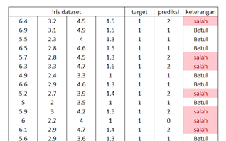
Bisa memprediksi pada proses training sebesar 94,7%
https://en.wikipedia.org/wiki/Extreme_learning_machine
http://www.ntu.edu.sg/home/egbhuang/

Sinopsis

References

Leave a Reply Cancel reply